Newton-Cotes formulas
The main objective is to numerically compute an integral. In order to do so, we shall introduce Lagrange interpolation polynomials, present the notions of quadrature rules and of exact quadrature rules on polynomial spaces. Finally, we shall define Newton-Cotes formulas and the particular cases of composite formulas for rectangles, trapezes and Simpson’s formula.
Let $f:[a,b] \rightarrow \mathbf{R}$ be a continuous function. The aim is to compute the following integral:
\[I(f)=\int_a^bf(x)dx\]We start by partitioning the interval $[a,b]$ into $n$ intervals $[x_i,x_{i+1}],i=0,\ldots,n-1$ with
\[a = x_{0} < x_{1} < \ldots < x_{n} =b.\]Therefore:
\[I(f)=\int_a^bf(x)dx=\sum_{i=0}^{n-1}\int_{x_i}^{x_{i+1}}f(x)dx\]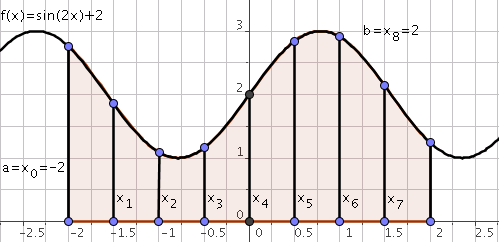
We then have to determine the following integral:
\[\int_{x_i}^{x_{i+1}}f(x)dx,i=0,\ldots,n-1.\]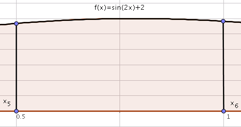
It is easy to switch to the interval $[-1,1]$ via the following substitution
\[t=2\frac{x-x_{i}}{x_{i+1}-x_{i}}-1\]or
\[x=\frac{x_{i+1}-x_{i}}{2}(t+1)+x_i\]therefore
\[\int_{x_i}^{x_{i+1}}f(x)dx=\frac{x_{i+1}-x_{i}}{2} \int_{-1}^{1}g_i(t)dt\]where
\[g_i(t)=f\left(\frac{x_{i+1}-x_{i}}{2}(t+1)+x_i\right),i=0,\ldots,n-1.\]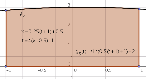
Quadrature rule
Let $g$ be a continuous function on $[-1,1]$. The application $J$
\[J:g \longmapsto \sum_{j=0}^p\omega_j g(t_j)\]is said to be a quadrature rule. The points defined by
\[-1\leq t_0 < t_1 < \ldots < t_p \leq 1\]are called points of integration of the quadrature $J$ and \(\omega_0,\omega_1,\ldots,\omega_p\) are the weights of the quadrature rule $J$.
The weights and the points of integration are chosen such that:
\[\int_{-1}^{1}g(t)dt\simeq\sum_{j=0}^p\omega_j g(t_j)\]Exact quadrature rule
Let $Q\in\mathbf{P}_q$ be the set of polynomials of degree at most equal to q. The quadrature rule $J$ is said to be exact in $\mathbf{P}_q$ if
\[\forall Q\in\mathbf{P}_q,\quad \int_{-1}^{1}Q(t)dt=J(Q)\]Alternatively stated, if
\[\forall Q\in\mathbf{P}_q,\quad \int_{-1}^{1}Q(t)dt=\sum_{j=0}^p\omega_j Q(t_j)\]Exact quadrature rule: Lagrange basis
Theorem.
Let $L_0,L_1,\ldots,L_p$ be the Lagrange-basis of $\mathbf{P}_{p}$ relatively to the points \(-1 \leq t_0 < t_1 < \ldots < t_p \leq 1.\)
We have the following equivalence:
\[J(g)=\sum_{j=0}^p\omega_j g(t_j)\mbox{ exact on } \mathbf{P}_{p} \Longleftrightarrow \omega_j=\int_{-1}^{1}L_j(t)dt,\quad j=0,1,\ldots,p.\]Newton-Cotes formula
Newton-Cotes’s method is obtained from the above mentioned methods for which the points $(x_i)_{i=0,\ldots,n}$ are equidistant
\[x_i=x_0+hi\]where $h=\frac{b-a}{n}$. This being so:
\[\begin{array}{ccl} \displaystyle\int_{x_i}^{x_{i+1}}f(x)dx &=& \displaystyle\frac{x_{i+1}-x_{i}}{2} \int_{-1}^{1}g_i(t)dt\\ &\simeq& \displaystyle\frac{h}{2}J(g_i)\\ &\simeq& \displaystyle\frac{h}{2}\sum_{j=0}^p\omega_j g_i(t_j)\\ &\simeq& \displaystyle\frac{h}{2}\sum_{j=0}^p\omega_j f\left(\frac{h}{2}(t_j+1)+x_i\right) \end{array}\]We can now approach $I(f)=\int_a^bf(x)dx$ by the composite formula $I_h(f)$:
\[\begin{array}{ccl} \displaystyle I(f)=\int_a^bf(x)dx&=&\displaystyle\sum_{i=0}^{n-1}\int_{x_i}^{x_{i+1}}f(x)dx\\ &\simeq&\displaystyle\frac{h}{2}\sum_{i=0}^{n-1}\sum_{j=0}^p\omega_j f\left(\frac{h}{2}(t_j+1)+x_i\right) \end{array}\]where
\[I_h(f)=\frac{h}{2}\sum_{i=0}^{n-1}\sum_{j=0}^p\omega_j f\left(\frac{h}{2}(t_j+1)+x_i\right)\]Following are some classical Newton formulas as well as the degree $p$ of $\mathbf{P}_{p}$.
| Degree p | Designation |
| 0 | Method of rectangles |
| 1 | Method of trapezes |
| 2 | Simpson’s method |
| 3 | 3/8 Simpson’s method |
| 4 | Boole’s method |
Method of rectangles
The method of rectangles is a one-point method. In this case, $p=0$ and $t_0=0$. Lagrange basis associated to $\mathbf{P}_{0}$ is
\[L_0(t)=1\]Consequently:
\[\omega_0=\int_{-1}^{1}L_0(t)dt=\int_{-1}^{1}dt=2\]The quadrature rule is defined by:
\[J(g)=\omega_0g(t_0)=2g(0)\]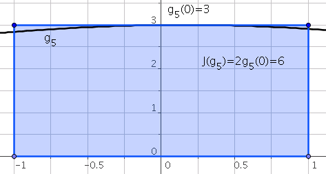
We thus have the composite rectangle formula:
\[I_h(f)=h \sum_{i=0}^{n-1}f\left(\frac{x_i+x_{i+1}}{2}\right)\]Method of trapezes
The method of trapezes is a two-point method. In this case, $p=1$ and $t_0=-1,t_1=1$. Lagrange basis associated to $\mathbf{P}_{1}$ is
\[L_0(t)=\frac{1-t}{2},L_1(t)=\frac{t+1}{2}\]Consequently:
\[\omega_0=\int_{-1}^{1}L_0(t)dt=1;\omega_1=\int_{-1}^{1}L_1(t)dt=1\]The quadrature rule is defined by:
\[J(g)=\omega_0g(t_0)+\omega_1g(t_1)=g(-1)+g(1)\]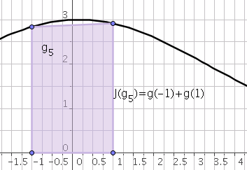
We thus have the composite trapezes formula:
\[I_h(f)=\frac{h}{2}\sum_{i=0}^{n-1}(f(x_i)+f(x_{i+1}))\]Simpson’s method
Simpson’s method is a three-point method. In this case, $p=2$ and $t_0=-1,t_1=0,t_2=1$. Lagrange basis associated to $\mathbf{P}_{2}$ is
\[L_0(t)=\frac{t^2-t}{2},L_1(t)=1-t^2,L_2(t)=\frac{t^2+t}{2}\]Consequently:
\[\omega_0=\int_{-1}^{1}L_0(t)dt=\frac{1}{3}; \omega_1=\int_{-1}^{1}L_1(t)dt=\frac{4}{3}; \omega_2=\int_{-1}^{1}L_1(t)dt=\frac{1}{3};\]The quadrature rule is defined by:
\[J(g)=\omega_0g(t_0)+\omega_1g(t_1)+\omega_2g(t_2) =\frac{1}{3}g(-1)+\frac{4}{3}g(0)+\frac{1}{3}g(1)\]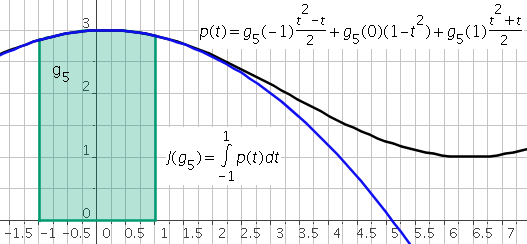
We thus have Simpson’s composite formula:
\[I_h(f)=\frac{h}{6}\sum_{i=0}^{n-1}(f(x_i)+4 f(\frac{x_i+x_{i+1}}{2}) +f(x_{i+1}))\]If you found this post or this website helpful and would like to support our work, please consider making a donation. Thank you!
Help Us